E12 Physical Systems Analysis:
Lab #4 Speed Bumps

Draft report due 1 week after lab date

Final report due 2 weeks after lab date (not including SB)

Lab Resources

Look at Prof. Cheever's resource for numerically solving ordinary differential equations, and use it as a resource when doing the lab.

• Numerical Solution of Differential Equations

Overall Objectives

For this lab you will be modeling the behavior of a car's suspension (one wheel of it, at least) using two different models. In addition to exploring the dynamics of a suspension system--and its relationship with speed bumps and other phenomena--you will be generating solutions using both Simulink and a numerical solution you will write in Matlab.

The final product of this lab should be a characterization of the behavior of a car under a variety of conditions. For example, after your analysis you should be able to provide a reasonable answer to the question, "What is the best speed bump design for keeping cars from going fast?".

As before, please work in groups of 2-3 people. Feel free to change lab groups if you wish.

Introduction

Model A

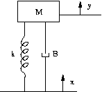
A simple model (model A) of a car's wheel and suspension is to consider the height of the road as a linear variable x, the height of the car as a linear variable y, with the two connected by a spring and a damper. This model is a poor approximation because it ignores the mass, damping and springiness of the tire. However, it does give some insight into how shocks are transmitted through the system.

This system is straightforward to analyze using a free-body diagram. The force exerted by the mass is equal to the force of the spring and damper. The force exerted by the spring is dependent upon the relative positions of x and y. Likewise, the force exerted by the damper is proportional to their relative velocities. If we assume that x and y are at their zero position when the system is at rest, then we can ignore the force of gravity acting on the mass, as it will be counteracted by an equal and opposite force generated by the spring.

Given this analysis, the equation of motion is:

Which we can simplify to the following notation:

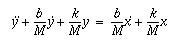
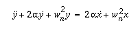
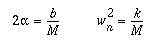
In short, the acceleration of the car, vertically, is a function of the height of the road, how quickly the road is changing, and the car's suspension parameters (spring and damping). Note that the horizontal velocity of the car plays a role because, for a bump in the road of a given size and shape, the horizontal velocity determines how fast the road is changing.

To model a nice bump in the road we can start with a simple function of s (distance along the road) with smooth derivatives.

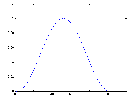
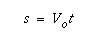
If we assume a constant horizontal velocity, then we can let:

The derivative of x is simple to compute:

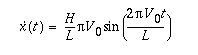
In case you were wondering why you really feel bumps in the road, consider a 2cm bump that is 10cm long--something like a filled-in pothole--that you go over at 55mph (~25m/s). At its maximum, the vertical velocity of the road reaches 0.2 * pi * 25m/s, or about 16m/s, which is about 35mph straight up.

Continuing that thought, from model A can we get a sense of what kind of shock the passengers are in for given a velocity and the bump profile?

An impulse (or shock) is defined as fdt. While it is difficult to estimate what dt will be for a given bump, we can appoximate it as one-half the time it takes to cross the bump--clearly there are no upward forces being applied after the half-way point. For the example case above--a 10cm bump at 25m/s--the time to get halfway across the bump is 2ms.

Now consider what effect the velocity and position change of the car will have on the car's acceleration--which is what the passengers feel. In 2ms, and with a 2cm high bump, the car's vertical position will change very little. If the position is not changing, then the vertical velocity of the car is not changing much either. Likewise, the change in the surface of the road is small as well, which means that, to a first approximation, the acceleration of the car is proportional to the velocity of the road, with the proportionality constant being b/M.

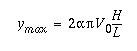
Rather than try to go out and measure the damping coefficient of the shock absorber of a car, we can actually make a fairly simple assumption to get at the value of b/M. First, consider that the spring is holding up the car in a steady state situation. Thus, we can write:

Therefore, if we know the initial offset of the wheel of a car, then we can estimate the natural frequency of the system. A typical offset for a wheel is 30cm (1ft), which gives a natural frequency of 5.7 rad/s, which is about 1Hz.

So how does this help us with estimating b/M? When designing a system, it is important to take into account the relationship between the natural frequency and the damping coefficient. When the damping frequency, alpha, is the natural frequency over the square root of two, then the system's recovery to zero displacement is the fastest possible with the least overshoot (but there is some overshoot). So if we assume the car's system is tuned to optimize response time and minimize overshoot, we can estimate b/M as about 8.

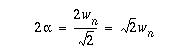
Now we can solve for the maximum acceleration using the relationship above. The end result is that the tiny 2cm bump provides a maximum acceleration of about 128m/s*s, or about 12 g's. Solving the system for the maximum velocity, and assuming the car reached that vertical velocity in the 4ms it took to cross half the bump, would provide an estimate of the impulse sent to the system. (Simulation reveals a maximum velocity of 0.7m/s, which for a 1000lb car produces an impulse force of 160,000N.)

As a final note, consider which term is passing on the shocks of the road to the passengers: the shock absorber term. Without the damper, the passengers wouldn't feel any shocks, just lots of bouncing.

Model B

For model B, a more realistic model of a suspension, we use two masses coupled with springs and dampers.

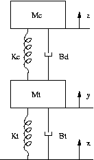
Model B is defined by two equations, one representing the forces on the car, the other representing the forces on the tire.

For this system, use the following parameters for the standard case:.

Tasks

1. Go measure the speed bumps on Whittier place using the 2x4 and dowel setup. Enter the data into a spreadsheet that can be loaded into Matlab.
2. Write an m-file function makeroad that generates a stretch of road that can be used by Simulink--it has to have both time and the function. The makeroad function should take as inputs the velocity of the car, and the height and length of the bump. It should return a single matrix consisting of two columns. The second column should be the road height, and the first column should be the time at which the car reaches that point in the road, assuming a constant velocity.
3. Build a Simulink model for Model A. Examine the response of the system to the following synthetic situations: A) an impulse bump that is 5cm high and 1cm wide, B) a standard speed bump 10cm high and 40cm long, and C) an approximation to the Whittier place speed bumps which are about 15cm high and 200cm long. Be sure to consider several velocities in your analysis, from very slow to reasonably fast.
4. Using Prof. Cheever's tutorial, write a 2nd order Runge-Kutta ODE solver for Model A. Compare your results to the output of Simulink.
5. Build a Simulink model for Model B. Examine the response of the system to each of the cases above. In addition, look at the response to a continuous stream of bumps. Be sure to look at a variety of speeds for all cases. Think about how you might check if the tires are in contact with the road at all times.
6. Using Model B, try to reduce the accelerations felt by the car for a small bump (2cm x 10cm long) at 65mph. Compared to the normal parameters, try to reduce the maximum acceleration by a factor of two. What combination of parameters would you use, given reasonable assumptions?
7. For both models, try the actual bump profiles from Whittier place. Compare the results to the cosine bump. Does the shape of the bump have an impact on the response of the car?
8. Using Model A, develop a criteria for the "nastiness" of a speed bump and determine what speed is best. Do you get similar results for model B?

Extensions

1. Try other parameters for Model B, including getting actual data on a variety of real car models.
2. Try other kinds of bumps. Can you make a more effective speed bump for an SUV (heavy, with bigger tires)?
3. Demonstrate why we use pneumatic tires, as opposed to solid tires.
4. Write a 4th-order R-K ODE solver and apply it to Model A and/or B.
5. Extend your analysis to two wheels of a car and the rigid body strung between them. What you are looking for in this case is the tilt of the car--the relative car positions--to determine where the back end of the car is relative to the road. Show how the maximum speed over the Whittier bumps is related to the length of the car's tail.
6. Compare the real data from a car and a truck going over the speed bump in front of Papazian. All of the data was captured on a video camera at 30fps. The first two columns are the (x, y) coordinates of the car, and the second two columns are the (x, y) coordinates of the wheel. The values are given in pixels, and you can convert to real distances using a value of 1.246 pixels/cm, or about 0.8 cm/pixel. Note that the speeds given are approximate. Knowing the distance conversion and frame rate, you should be able to calculate the real speed of the vehicle.
• car1.dat (6 mph, 30fps)
• car2.dat (9 mph, 30fps)
• car3.dat (12 mph, 30fps)
• car4.dat (15 mph, 30fps)
• truck1.dat (5 mph, 30fps)
• truck2.dat (10 mph, 30fps)
• truck3.dat (12 mph, 30fps)
• truck4.dat (15 mph, 30fps)

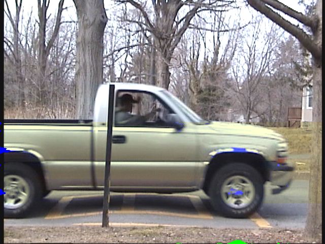
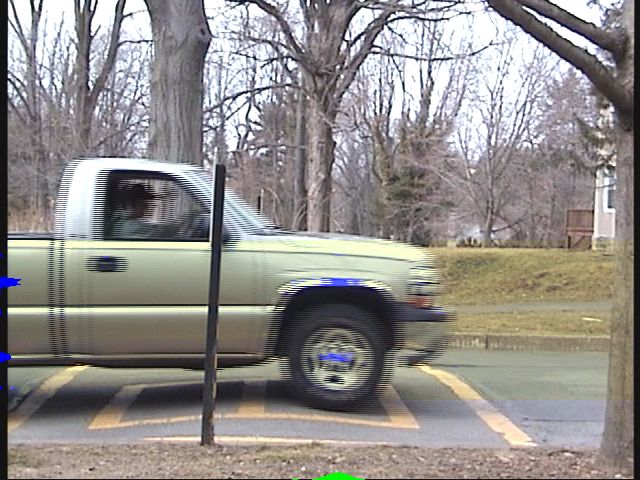
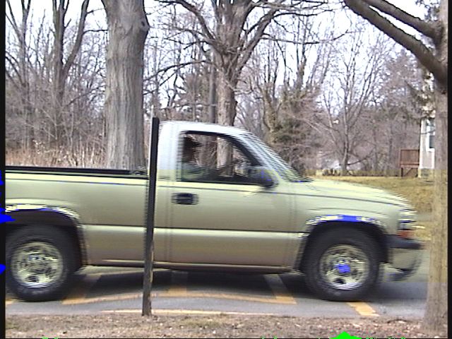
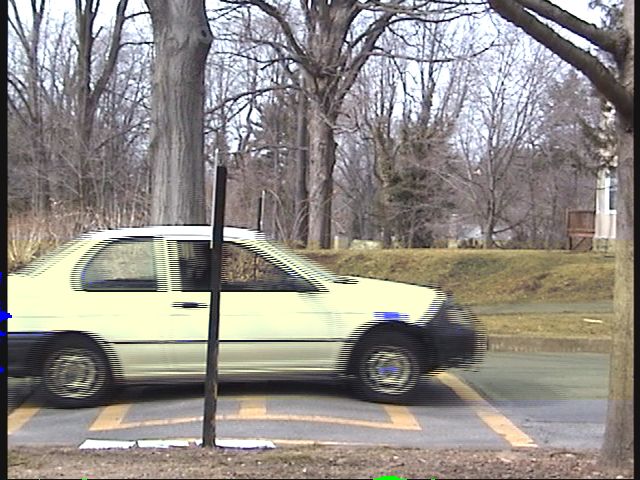
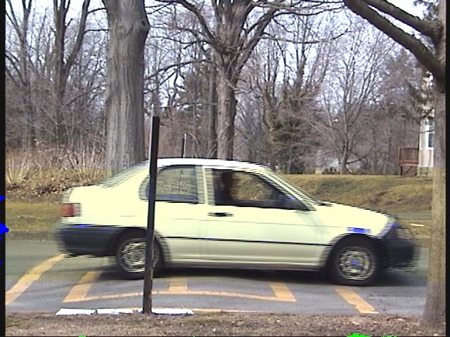
Here are some examples of the pictures the data came from (click on an image for a closeup).

Writeup

Make a web page that shows your models, experiments, and conclusions. Organize it so that there is a main page that gives a discription of the task and a summary of all the cases you explored. This page should also include a brief discussion of what you discovered and your conclusions, and it needs to have any extra derivations, outside information, or calculations you made. From the main page link each of the cases, as appropriate. You should combine cases to make a point--for example, combine the different velocity cases for a given speed bump shape.

Send the URL to Prof. Maxwell when it is ready for viewing.