E12 Physical Systems Analysis:
Lab #3 Double Trouble

Draft report due 1 week after lab date

Final report due 2 weeks after lab date (not including SB)

Lab Resources

It will behoove you to look at the following resources before coming to the lab.

• Numerical Solution of Differential Equations
• Using Simulink to Solve Ordinary Differential Equations

Overall Objectives

For this lab we will be modeling the behavior of a system of two loosely coupled pendulumns using two different methods: an analytic method, and an analog computer simulation method (Simulink).

As before, please work in groups of 2-3 people. Feel free to change lab groups if you wish.

Introduction

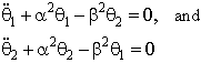
Draw free body diagrams for the system and set up the simultaneous differential equations describing the system. If you assume no applied forces, no damping, and small angles (what determines how small?), you can write a set of coupled second order differential equations:

              (eq 1)

where you should define a and b in terms of m, g, k, L, and r.  If you assume a solution of the form

          (eq 2)

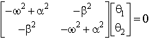
the equation can be put in the form:

             (eq 3)

or

          (eq 4)

There are only certain values of w for which this equation will be true.  These are called the eigenvalues of the system, and are determined by solving for the determininant of the "M" matrix and setting this to zero:

             (eq 5)

In our system this yields four eigenvalues:

              (eq 6)

where

            (eq 7)

These two frequencies represent the two "modes" of the system.  Note that if either of these modes is put back into equation 3, it determines a relationship between q₁ and q₂.  For example if we let

            (eq 8)

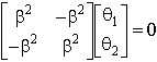
equation 3 becomes

               (eq 9)

which has the solution

                 (eq 10)

which is often exressed as

              (eq 11)

The vector in (11) is called an eigenvector of the system that is associated with w_p. This corresponds to the mode in which the two pendula are swinging in phase with each other, and the spring has no effect.  The other mode corresponds to the case where the pendula are out of phase with each other so

         (eq 12)

and

         (eq 13)

Any motion of the pendula starting from inital conditions with zero velocity, can be described as a sum of these two modes:

               (eq 14)

(if the velocity is non-zero, sine functions need to be added).   The unknown coefficients Kp and Kc are determined by initial conditions.

With a single non-zero initial condition, q₁(0)=q₀, it can be shown that the solution reduces to

            (eq 15)

The right-hand side of Equation 15  follows from a trigonometric identity. You should show that:

        (eq 16)

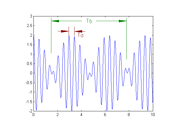
In the lab this will produce a response similar to that shown below. By measuring T_a and T_b (preferably over several periods) it is possible to determine w_a and w_b.

Setting Up

For this lab you will need the following.

• The pendulum apparatus (there's only one, so share).
• A computer with a NIDAQ board.

Tasks

1. Measure L and r on the physical system.

2. Using the programs you wrote for lab 1, capture data from one pendulum from three different runs.
   • Case 1: start the pendula with equal and opposite initial conditions.

   • Case 2: start the pendula with identical initial conditions.

   • Case 3: start the pendula with only one pendulum having a non-zero initial condition.

3. Determine w_a and w_b from the time series plot (as shown above). Calculate w_c and w_p based on your measurements using (16).
4. Use the Fourier transform to analyze your data and calculate w_p and w_c. Before taking the fft() of your data you should multiply the time domain signal by a Hamming window of the same size. You can use the hamming(N) function to generate a Hamming window of size N. In your lab writeup, comment on any differences in your estimates of w_c and w_p using the two methods. Note that, since the Fourier transform is linear, it sees the form of the solution given in (14), which is the sum of the two mode frequences, not the multiplication of the frequencies in (15). In your lab report, write down what you expect the Fourier transform of the data to look like, and comment on whether it matched your expectations.
5. Determine k (spring constant) from these results. The mass of each weight is 1.5kg.

6. Plan your analog computer model and implement it on Simulink.
   • Start with a pair of integrators (1/s units) for each angle.
   • Solve the state equations for the accelerations (second derivatives) in terms of the first and zeroth order terms.
   • The integators give you the lower order terms, which just need to be connected with gain and summation units to generate the acceleration signal.
7. Compare your captured data with your analytic model and Simulink for each of the three starting situations: theta equal, theta opposite but equal, and one theta non-zero.

Extensions

1. Capture data from some other runs with different initial conditions and see if they still compare well to the theoretical solutions.
2. Determine the amount of friction in the bearings of the system. If you choose to do this, explain your method carefully.
3. Try writing a Runge-Kutta differential equation solver and compare the results to your system. The link at the top of the lab gives you the information you need to begin.

Lab Report