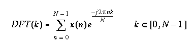
Discrete Fourier Transform definition for N samples

Graphs and results from parts 1-8 due 1 week after lab date
Final report due 2 weeks after lab date
This lab will give you some hands-on experience with the Fourier transform, which is one of the most useful tools in signal processing and analysis. We will be working with 1D Fourier Transforms to clean up noisy speech.
In order to process both speech and images on a computer, they must first be sampled at discrete intervals. The sampling frequency--the inverse of the sampling interval--is determined by the characteristics of the signal being measured.
Human speech, for example, uses a range of frequencies from approximately 200Hz to 10kHz, although the most important range is below 5kHz. The Nyquist criterion tells us that we must sample a signal at a frequency at least twice that of the frequency of the signal we want to measure. Otherwise, aliasing results, which is the signal folding back on itself in the frequency domain. Because of the Nyquist criterion, speech is usually sampled at no less than 8kHz. High quality CD music is sampled at 44kHz, which captures pretty much the whole range of human hearing abilities. For this lab, we will sample the speech at 11.025kHz.
We would like to execute a Fourier transform [FT] on our data in order to analyze and process it. Because our data is a string of samples, however, we cannot treat it as a continuous signal when executing a Fourier analysis. Instead, we must use the discrete Fourier transform [DFT]. The DFT executes the Fourier Transform of a finite-length sequence of complex points.
Discrete Fourier Transform definition
for N samples
For real-valued input data like speech samples, the value of the complex part of each sample is zero.
The most important difference between the DFT and the continuous FT is that the DFT works on a finite set of samples. From the point of view of the DFT, however, the finite set of samples represents one "example" of an infinitely repeated sequence of samples. In other words, the signal you are actually analyzing is the signal you would get by repeating the sequence of samples, with x(0) coming after x(N-1), infinitely in both directions (positive and negative).
Likewise, DFT(-k) = DFT(N-k), which means the negative frequency portion of the spectrum appears in the top half of DFT(k) in locations k = N/2 to k = N-1. Normally, only the positive frequences are plotted when viewing the spectrum.
A second major difference between the DFT and the continuous FT is that, in order to extract a finite sample to analyse, we have to cut out a window of our signal of interest. For example, we may want to analyze a half second of speech sampled at 11kHz from a sample that is 3s long. In order to extract the sample we are, in effect, multiplying the 3s sample by a rectangular window function that has the value 1 within the half-second period of interest and 0 otherwise.
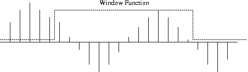
This doesn't seem like a real big deal until you realize that multiplication in the time domain is equal to convolution in the frequency domain. This means that the spectra of the windowing function and the signal of interest will be convolved--in other words pretty badly mixed up.
Now there is a function that acts as the identity in convolution: the delta function. If you convolve a delta function centered at 0 with another function g(n) you get back g(n). Since the inverse FT of the delta function at 0 is a uniform value over all time (a DC signal), this is the same as using a window of infinite length. This should make sense, since a window of infinite length basically gets you back to the continuous FT, which doesn't have to use windows.
So where is this going? Well, what we want to find is a windowing function that looks like a delta function in the Fourier domain so that it doesn't mess up our signal analysis too much. A square window, unfortunately, looks like a large lobe in the center and many smaller lobes to the side. While the center lobe is fairly thin and peaked--similar to a delta function--the side lobes mean that the convolution will "leak" information from one frequency to many others.
The signal processing community has studied this problem for a long time and there are several windowing functions that are in common usage. One of the most commonly used is the Hamming function, which looks like a Gaussian that goes towards zero at the edges of the window. The Hamming window (see definition below) has a spectrum that is a single lobe, 46 percent wider than a rectangular window, but with virtually no side lobes. Thus, the effect of the Hamming window is to blur the Fourier spectrum a bit, but without the wider "leakage" that occurs with a rectangular window. This is the price you pay for the uncertainty that comes with executing an FT on a finite sequence of samples.
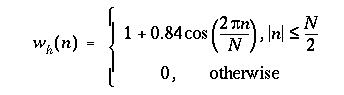
Hamming Window Function for N samples
One of the major uses of the Fourier Transform in signal analysis is to either detect or remove repeating signals. We will be doing the latter in this lab and the former in a follow-up lab later on.
In particular, for this lab we will be trying to remove a 400Hz signal from a captured speech signal. In the time domain, the captured signal can be represented as y(t) = s(t) + n(t), where s(t) is the speech and n(t) is the noise. In the Fourier domain, the signal is Y(w) = S(w) + N(w). While it may seem like we haven't gained much in the process, in the Fourier domain the periodic noise signal and its harmonics are compressed into a few points representing particular frequencies. If we reduce the value of these points in the Fourier domain and then take the inverse DFT, we should get a much cleaner signal.
Now to work.
For this lab you will need the following items:
We will be using matlab for this exercise, so sharpen up your m-file skills.
[N, trash] = size(corrupt);
To set the noise sample to N data points, use:noise = noise(1:N);
To take the DFT of the samples use the function fft:noiseFFT = fft(noise);
The first time through this process, don't worry about the Hamming window, especially if your phrases begin and end during relative silence.DELTAF = 1 / (N * Ts)
where N is the number of elements in the speech sample and Ts is time between samples (1 / fs). Then create a variable FREQ that goes from 0 to N*DELTAF. If DELTAF is defined as above and the sampling frequency (hopefully 11025) is defined as FS, then you can do this using the following expression:FREQ = 0:DELTAF:FS/2;
FREQ = FREQ';
The second statement is necessary to convert the FREQ matrix from a row vector to a column vector.
Now you can plot the FTs versus FREQ and see the spectra of the three samples. For example, to plot the magnitude of the positive half of the noise spectrum, use the following:
plot(FREQ(1:N/2), abs(noiseFFT(1:N/2)));
You may want to make an m-file that does all of the steps so for you automatically. Look for the 400Hz signal in the noise sample and its harmonics.
npc = abs(noiseFFT) .* abs(noiseFFT);
In the m-file, calculate the power spectrum and then subtract the noise from the signal. Since a power spectrum must be positive, clip any negative results to zero or invert their sign (choose one method). Use a for loop and an if statement.
Then, using the new magnitude from the power spectrum and the phase of the corrupt phrase, recreate the complex number for each sample. The m-file should return a cleaned up signal.
The tricky part here is recreating the Fourier transform, which is a series of complex numbers. In part one, you subtract the power spectrum of the noise from the power spectrum of the corrupted speech, which results in a new power spectrum. However, the power spectrum does not represent the phase of the signal. To get a complete cleaned up signal, you need both parts. The output signal should have the same phase as the corrupted speech signal, so you can rebuild the magnitude and phase from the new power spectrum and the old phase information.
The writeup for this lab is not totally formal, but should be structured. You may turn it in either as hard copy or as a URL (web page). Please include the following sections in your writeup.