E28/CS82 Mobile Robotics: Homework

Homework 1

Due Thursday, 1 February 2007

  1. Discuss how motion planning differs from collision avoidance.
  2. Under what assumptions is it reasonable to assume that a wheeled robot is a two-dimensional object moving freely in a plane?
  3. Give two examples of a non-holonomic robot and explain why they are non-holonomic. Why do we use non-holonomic vehicles?
  4. You have a robot that can move at a maximum velocity of 1m/s, with the ability to accelerate at +/- 2m/s. You have sonar sensors that are useful between 0.5m and 3m, and it takes you 50ms to decide upon and implement an action. How often do you have to sample the sonars to ensure that you are not going to run into a stationary obstacle?
  5. Using the same robot as above, how often do you have to sample the sonars and make decisions to ensure that you do not run into an obstacle going 1m/s towards the your robot? What, therefore, is the maximum number of computer operations you can execute in a single sense-act cycle on a 500MHz computer, assuming 1 operation per clock cycle. This is an estimate of how complex a program you can run while navigating in real time. Divide this number by 86,400 to get an upper bound on the number of image processing operations you can use on half-size video. If N is the number of pixels (86,400) Is it possible to use any image processing operations that are more complex than O(N)?

Homework 2

Due Thursday, 15 February 2007

Download the kalman1d.c and gaussDist.c source files. Then you need to fill in the Kalman filter update equations in the middle of the main loop. You will also need to initialize the H, Q, and phi variables, as appropriate. Use a scalar state variable to begin with, storing and updating only position. Any change to to a non-zero velocity will need to be modeled as process noise (Q).

  1. Try out different combinations of sensor noise and estimated sensor noise (R, in the Kalman filter equations). Plot the output, which is spewed to the data file, and look at the different responses for different values of Q and R. Learn gnuplot.
  2. Make the system use a 2-element state vector (position and velocity), but still only a single measurement vector. The Kalman gain equation should still be a scalar equation, but the state update matrix will be 2x2, as will the system covariance matrix P. Compare the results for different levels of noise.

    Hand in a copy of your code as well as a few plots of the sensor readings and the Kalman state values. Summarize your observations about what happens for different values of Q and R. Also observe how the various Kalman filter parameters affect the behavior of the proportional control system.

    Homework 3

    Due Tuesday, 27 February 2007

    Do this exercise with a partner in the Kohlberg or Science Center coffee bar areas.

    1. Pick a starting location on one side of the room, and a goal point on the far side of the room. Navigate your way to the goal point as quickly as you can while still walking while your partner notes the strategy you use to move around obstacles. In particular, note how far away from obstacles you pass, and how and when you change direction. Switch and have your partner repeat the exercise. Try not to consciously manage your movements.
    2. Repeat the exercise, but this time try to stay equidistant from obstacles. In other words, try to keep the distance to obstacles on either side of you the same. Comment on whether it felt natural to follow this strategy and how it affected your speed.
    3. Finally, close your eyes and have your partner adjust the obstacles (probably chairs) such that there are dead ends and blocked paths between you and your goal point. Then put something over your eyes, or shade them so that you can see at most a meter or so ahead of you. Try to get to your goal point as fast as possible without going over or through any obstacles. Have your partner note your strategy. Then switch roles.
    4. Based on your exercises, comment on strategies for navigation and planning in complex environments. What was natural, what worked, and what didn't?

    Homework 4

    Due Thursday, 5 April 2007

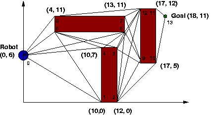
    1. Code up Dijkstra's algorithm and test it on the simple visibility graph below. A simple way to represent the visibility graph is to use an array to represent the vertices, and a 2D matrix to represent whether a connection exists between any two vertices. You can use this file to get started. It defines some basic data types as well as the graph itself. Run your algorithm for both the goal point specified below and for the goal point (18, 7). Report the complete path in both cases along with the cost (distance traveled) from the start point to each intermediate point and to the final goal.